Read the maps and uncertainty plots

Shaowen Ye

Fit a small example

A component plane shows one fitted map. It cannot show how much the result changes across resampled data, grid sizes and random starts. We therefore read the map together with the ensemble plots.

library(SOMevidence)

dat <- simulate_som_scenario(
  "clusters",
  n = 120,
  p = 6,
  seed = 201
)

resamples <- som_resamples(
  dat,
  method = "subsample",
  repeats = 3,
  seed = 202
)

spec <- som_spec(
  grids = list(c(4, 3), c(5, 4)),
  seeds = c(203, 204),
  rlen = 50,
  k = 2:5
)

workflow <- run_som_workflow(
  dat,
  spec,
  resamples,
  cross_models = c("kmeans", "ward")
)

fit_id <- workflow$ensemble$fits[[1]]$id

Look at one map

plot_som_plane(
  workflow$ensemble,
  fit_id = fit_id,
  variables = colnames(dat$layers$environment)[1:4]
)

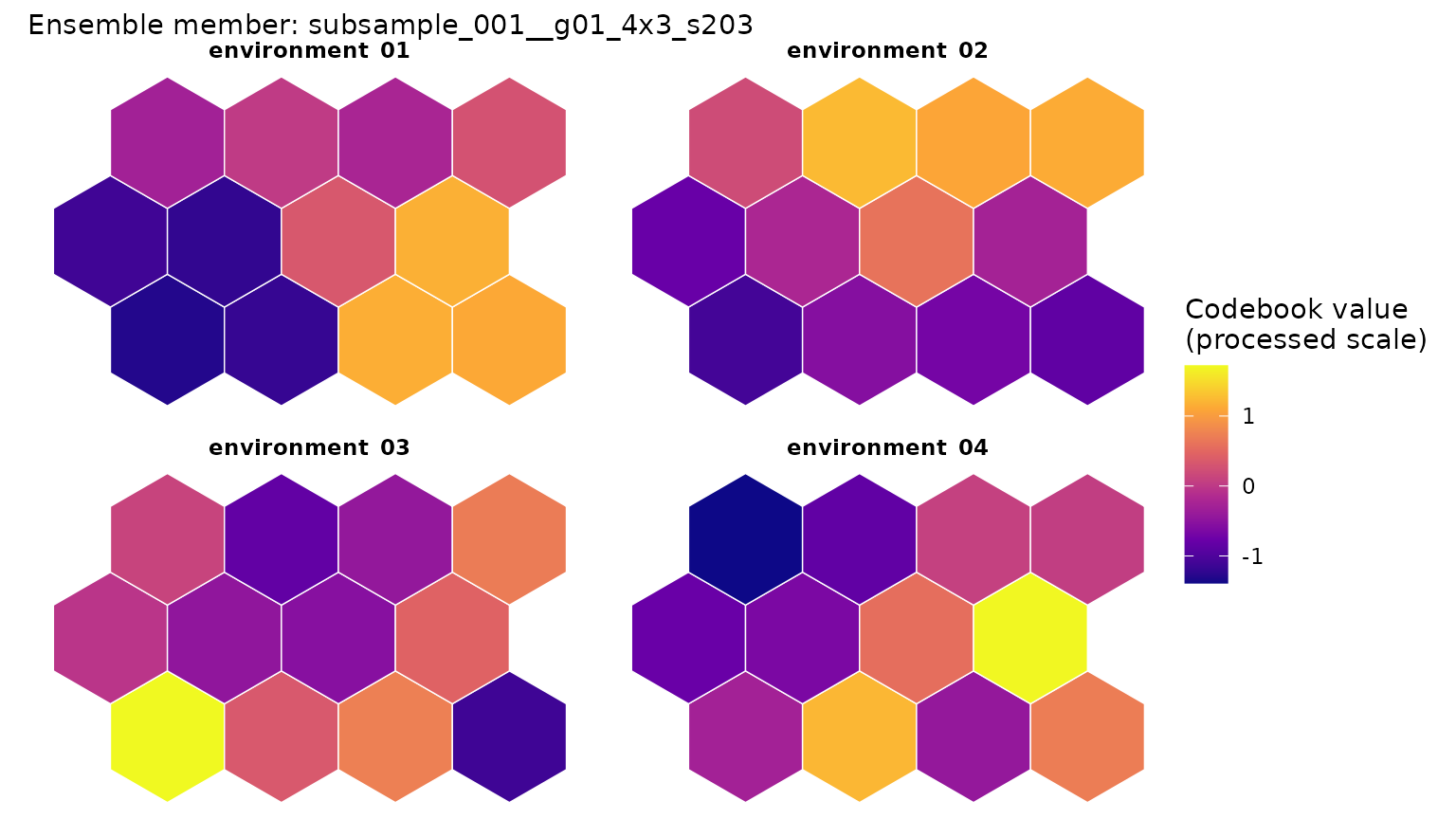
The colours show codebook values after the preprocessing used for this fit. The subtitle identifies the ensemble member. If more than one map is available, fit_id is required so that the displayed map is unambiguous.

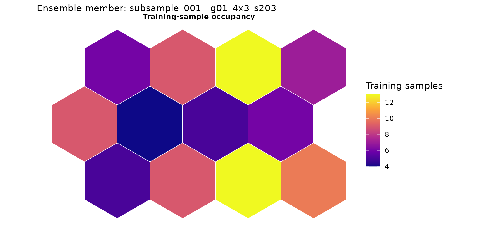
Two companion views help explain the map:

plot_som_plane(
  workflow$ensemble,
  type = "occupancy",
  fit_id = fit_id
)

plot_som_plane(
  workflow$ensemble,
  type = "neighbour_distance",
  fit_id = fit_id
)

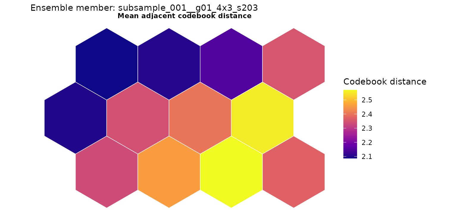
Occupancy shows how many observations use each map unit. Neighbour distance shows changes between adjacent codebook vectors. Neither view tells us whether a hard classification is stable.

Put ensemble evidence beside the map

plot(workflow$audit)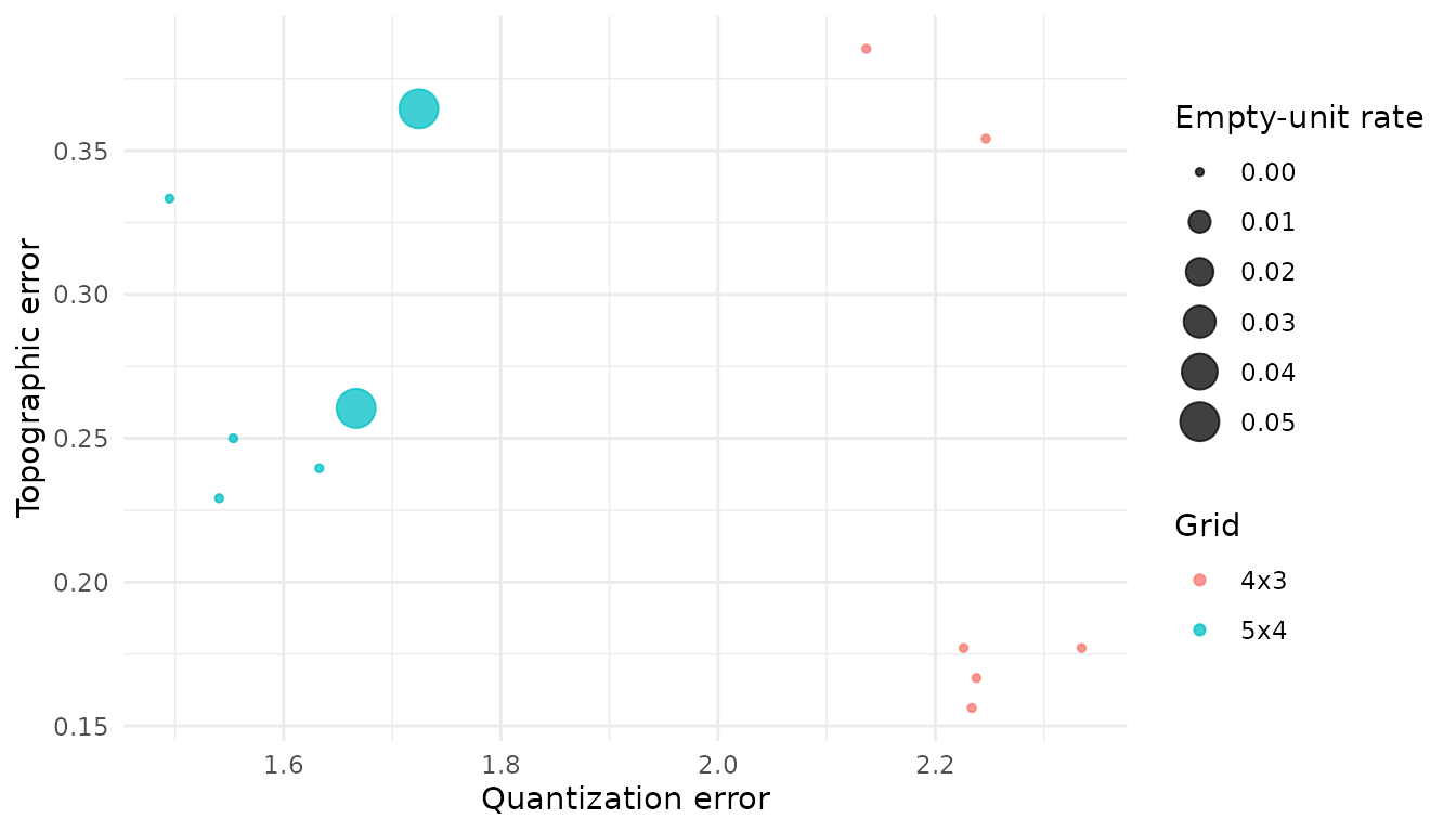

plot(workflow$partitions)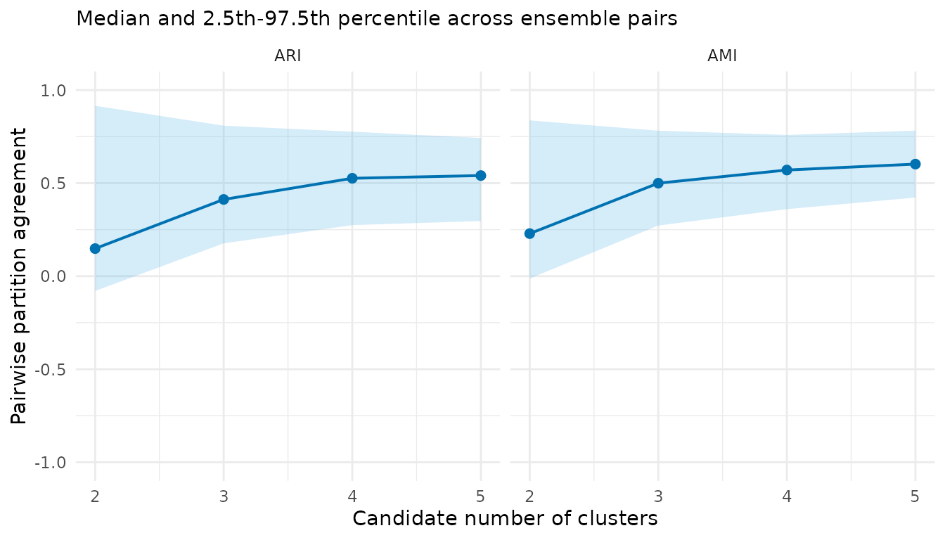

The first plot summarizes representation diagnostics and fit success. The second shows how candidate partitions vary across the ensemble. Read the displayed intervals and coverage rather than choosing a result from colour or visual separation alone.

Find uncertain samples

consensus_k3 <- workflow$consensus$k3
plot(consensus_k3)
#> Warning: Removed 3 rows containing missing values or values outside the scale range
#> (`geom_point()`).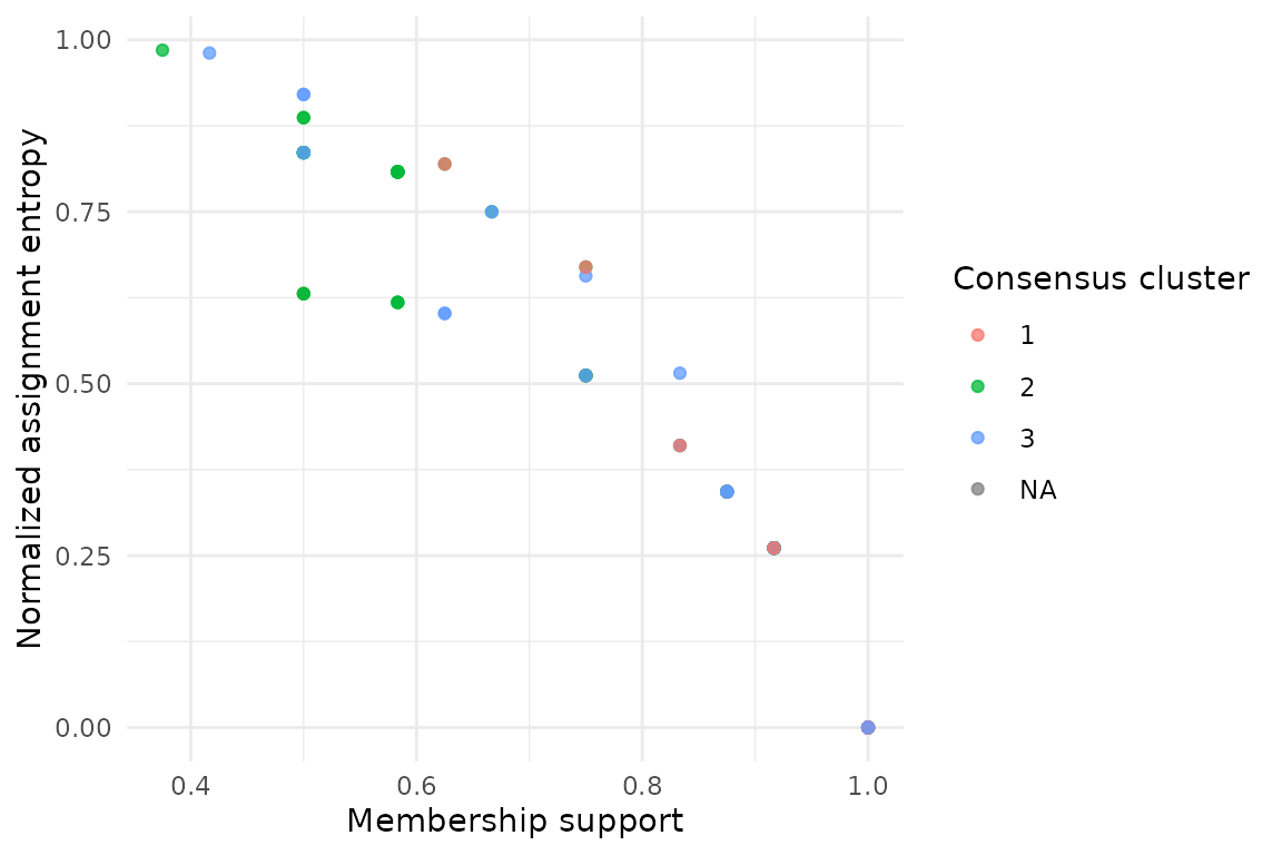

consensus_k3$cluster_summary
#>   cluster median_jaccard jaccard_q025 jaccard_q975
#> 1       1      0.8573589    0.4310345    0.9677419
#> 2       2      0.5827922    0.3043478    0.9166667
#> 3       3      0.6866071    0.3921569    0.8285714

Membership support and assignment entropy show where the repeated fits agree and where they do not. A consensus label is still conditional on the chosen data, preprocessing, ensemble and k.

Compare reference methods

plot(workflow$cross_comparison)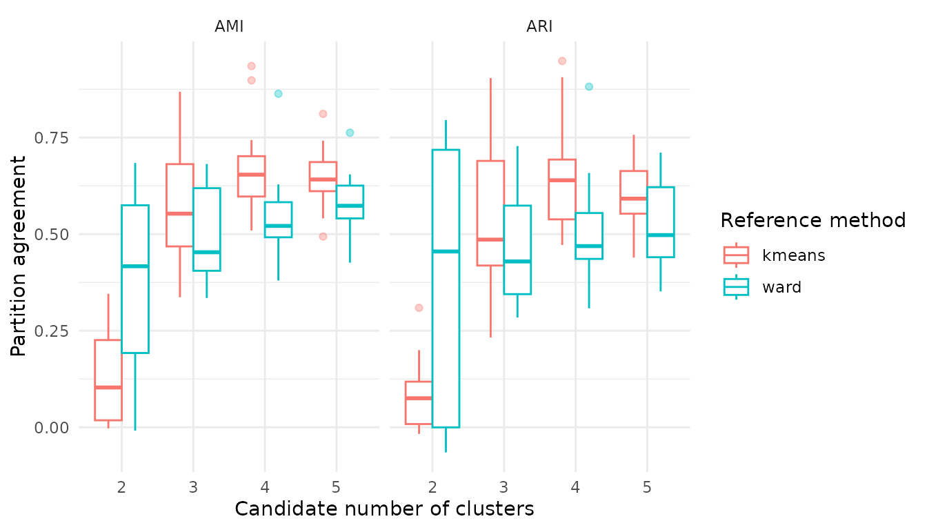

This plot shows agreement with the prespecified reference methods. It does not rank the methods or turn agreement into accuracy.

For a report, keep at least three views together: one clearly identified map, the ensemble representation diagnostics and the partition or consensus evidence. This is more informative than a single attractive SOM figure.