Worked example: Palmer penguin morphology
Shaowen Ye
Source:vignettes/v05-palmer-penguins.Rmd
v05-palmer-penguins.RmdThe question
This example asks how reproducibly a SOM represents and partitions four penguin body measurements. Species is kept as an external label and is inspected only after fitting.
The example does not assume that a SOM class is a species. Morphology overlaps among species and does not define taxonomy by itself.
The palmerpenguins package distributes the data under
CC0. Its documentation provides the original data source and citations.
If the optional package is not installed, this vignette displays the
code without running it.
Prepare the data
library(SOMevidence)

raw <- palmerpenguins::penguins
variables <- c(
  "bill_length_mm",
  "bill_depth_mm",
  "flipper_length_mm",
  "body_mass_g"
)

keep <- stats::complete.cases(
  raw[, c(variables, "species", "year")]
)
penguins <- raw[keep, , drop = FALSE]
sample_ids <- sprintf("penguin_%03d", seq_len(nrow(penguins)))

morphology <- som_data(
  x = penguins[, variables],
  id = sample_ids,
  time = penguins$year,
  domain = factor(penguins$year),
  external_label = stats::setNames(
    as.character(penguins$species),
    sample_ids
  )
)
morphology
#> <som_data>
#>   samples: 342
#>   layers : 1
#>   id source: provided
#>     - data: 4 variables, 0.0% missing
#>   design : time, domain, external_label
Stable IDs link results back to observations. Year defines the transfer domain. Species remains outside the training matrix.
Leave out one year at a time
Each split trains on two sampling years and assesses the third. Preprocessing is estimated from the training years only.
year_splits <- som_resamples(
  morphology,
  method = "leave_domain_out",
  domain = "domain"
)

spec <- som_spec(
  grids = list(c(4, 3), c(5, 4)),
  seeds = c(41, 42),
  rlen = 50,
  k = 2:4
)

year_splits
#> <som_resamples>
#>   method    : leave_domain_out
#>   splits    : 3
#>   unique analysis sets: 3
#>   analysis  : 223-233 rows
#>   assessment: 109-119 rows
The ensemble is intentionally small so that the vignette builds quickly.
Fit and inspect the workflow
workflow <- run_som_workflow(
  morphology,
  spec,
  year_splits,
  preprocess = som_preprocess(
    center = TRUE,
    scale = TRUE
  ),
  cross_models = c("kmeans", "ward")
)
summary(workflow)
#> <summary.som_workflow>
#>   SOM success: 12 / 12
#>   consensus  : 2 computed; 1 not_computed
#>     - k=2: computed; complete=yes; assignment=100.0%; labels=100.0%; replicated=100.0%
#>     - k=3: computed; complete=yes; assignment=100.0%; labels=100.0%; replicated=100.0%
#>     - k=4: not_computed
#>   reference methods:
#>     - kmeans: 9 expected, 9 succeeded, 0 failed, 0 warnings, 100.0% success
#>     - ward: 9 expected, 9 succeeded, 0 failed, 0 warnings, 100.0% success
Read the evidence streams separately.
workflow$audit$grid_summary
#>    grid xdim ydim n_fits median_quantization_error median_topographic_error
#> 1 4 x 3    4    3      6                 0.4097716               0.03587444
#> 2 5 x 4    5    4      6                 0.3031615               0.07908158
#>   median_empty_unit_rate
#> 1             0.04166667
#> 2             0.05000000
workflow$partitions$stability
#>   k    scope n_pairs n_partitions n_complete_partitions min_observed_clusters
#> 1 2 analysis      66           12                    12                     2
#> 2 3 analysis      66           12                    12                     3
#> 3 4 analysis      66           12                    12                     4
#>   n_pairs_evaluable median_joint_n median_joint_coverage median_ari  ari_q025
#> 1                66            119             0.3479532  1.0000000 1.0000000
#> 2                66            119             0.3479532  0.9464004 0.5837585
#> 3                66            119             0.3479532  0.6341304 0.4433956
#>   ari_q975 median_ami  ami_q025 ami_q975
#> 1        1  1.0000000 1.0000000        1
#> 2        1  0.9190143 0.6945523        1
#> 3        1  0.7661608 0.6524782        1
workflow$consensus$k3$cluster_summary
#>   cluster median_jaccard jaccard_q025 jaccard_q975
#> 1       1      0.9809524    0.5384615            1
#> 2       2      1.0000000    1.0000000            1
#> 3       3      0.9583333    0.4545455            1
workflow$cross_comparison$summary
#>      scope method k n_comparisons median_ari  ari_q025  ari_q975 median_ami
#> 1 analysis kmeans 2            12  1.0000000 1.0000000 1.0000000  1.0000000
#> 2 analysis   ward 2            12  1.0000000 1.0000000 1.0000000  1.0000000
#> 3 analysis kmeans 3            12  0.7893609 0.7108707 0.8804393  0.8086069
#> 4 analysis   ward 3            12  0.9646697 0.6203559 0.9876968  0.9441975
#> 5 analysis kmeans 4            12  0.6293081 0.5052421 0.7871324  0.7221508
#> 6 analysis   ward 4            12  0.9379016 0.4740153 0.9732182  0.9149813
#>    ami_q025  ami_q975
#> 1 1.0000000 1.0000000
#> 2 1.0000000 1.0000000
#> 3 0.7533403 0.8767339
#> 4 0.7233573 0.9774167
#> 5 0.6564826 0.8359577
#> 6 0.6512134 0.9682041

transfer <- audit_transfer(workflow$ensemble)
transfer$metrics
#>                                     id               split_id grid_id seed
#> 1  leave_domain_001_X2007__g01_4x3_s41 leave_domain_001_X2007       1   41
#> 2  leave_domain_001_X2007__g01_4x3_s42 leave_domain_001_X2007       1   42
#> 3  leave_domain_001_X2007__g02_5x4_s41 leave_domain_001_X2007       2   41
#> 4  leave_domain_001_X2007__g02_5x4_s42 leave_domain_001_X2007       2   42
#> 5  leave_domain_002_X2008__g01_4x3_s41 leave_domain_002_X2008       1   41
#> 6  leave_domain_002_X2008__g01_4x3_s42 leave_domain_002_X2008       1   42
#> 7  leave_domain_002_X2008__g02_5x4_s41 leave_domain_002_X2008       2   41
#> 8  leave_domain_002_X2008__g02_5x4_s42 leave_domain_002_X2008       2   42
#> 9  leave_domain_003_X2009__g01_4x3_s41 leave_domain_003_X2009       1   41
#> 10 leave_domain_003_X2009__g01_4x3_s42 leave_domain_003_X2009       1   42
#> 11 leave_domain_003_X2009__g02_5x4_s41 leave_domain_003_X2009       2   41
#> 12 leave_domain_003_X2009__g02_5x4_s42 leave_domain_003_X2009       2   42
#>    n_analysis n_assessment n_analysis_mapped n_assessment_mapped
#> 1         233          109               233                 109
#> 2         233          109               233                 109
#> 3         233          109               233                 109
#> 4         233          109               233                 109
#> 5         228          114               228                 114
#> 6         228          114               228                 114
#> 7         228          114               228                 114
#> 8         228          114               228                 114
#> 9         223          119               223                 119
#> 10        223          119               223                 119
#> 11        223          119               223                 119
#> 12        223          119               223                 119
#>    analysis_mapping_coverage assessment_mapping_coverage
#> 1                          1                           1
#> 2                          1                           1
#> 3                          1                           1
#> 4                          1                           1
#> 5                          1                           1
#> 6                          1                           1
#> 7                          1                           1
#> 8                          1                           1
#> 9                          1                           1
#> 10                         1                           1
#> 11                         1                           1
#> 12                         1                           1
#>    median_analysis_distance median_assessment_distance distance_ratio
#> 1                 0.2994931                  0.5238194       1.749020
#> 2                 0.2900610                  0.5160382       1.779068
#> 3                 0.2358949                  0.4119525       1.746339
#> 4                 0.2222224                  0.3937044       1.771669
#> 5                 0.3294059                  0.3878611       1.177456
#> 6                 0.3294059                  0.3473567       1.054494
#> 7                 0.2279949                  0.3130662       1.373128
#> 8                 0.2328458                  0.3139906       1.348492
#> 9                 0.2692782                  0.3872812       1.438220
#> 10                0.2732061                  0.4286799       1.569072
#> 11                0.2195664                  0.3602205       1.640599
#> 12                0.2312665                  0.3528038       1.525529
#>    unoccupied_unit_rate
#> 1           0.000000000
#> 2           0.000000000
#> 3           0.000000000
#> 4           0.000000000
#> 5           0.008771930
#> 6           0.000000000
#> 7           0.000000000
#> 8           0.000000000
#> 9           0.000000000
#> 10          0.008403361
#> 11          0.016806723
#> 12          0.016806723
plot(workflow$audit)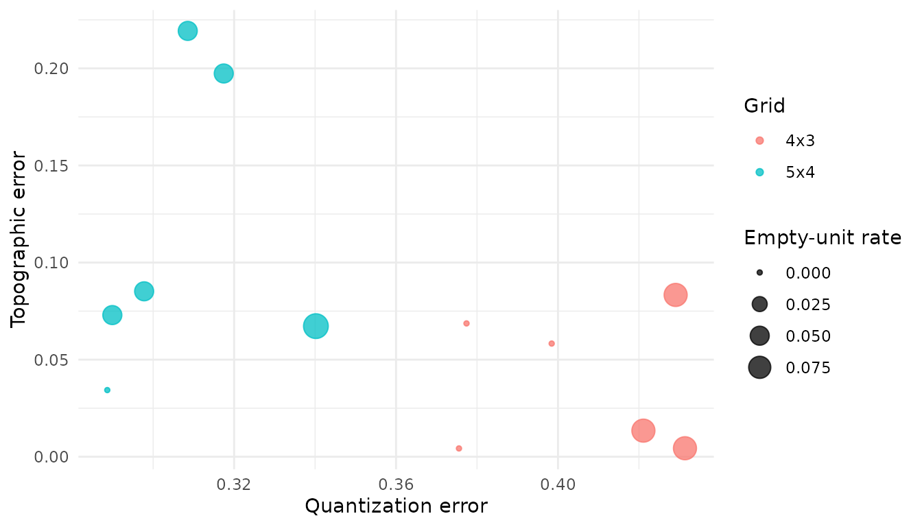
plot(workflow$partitions)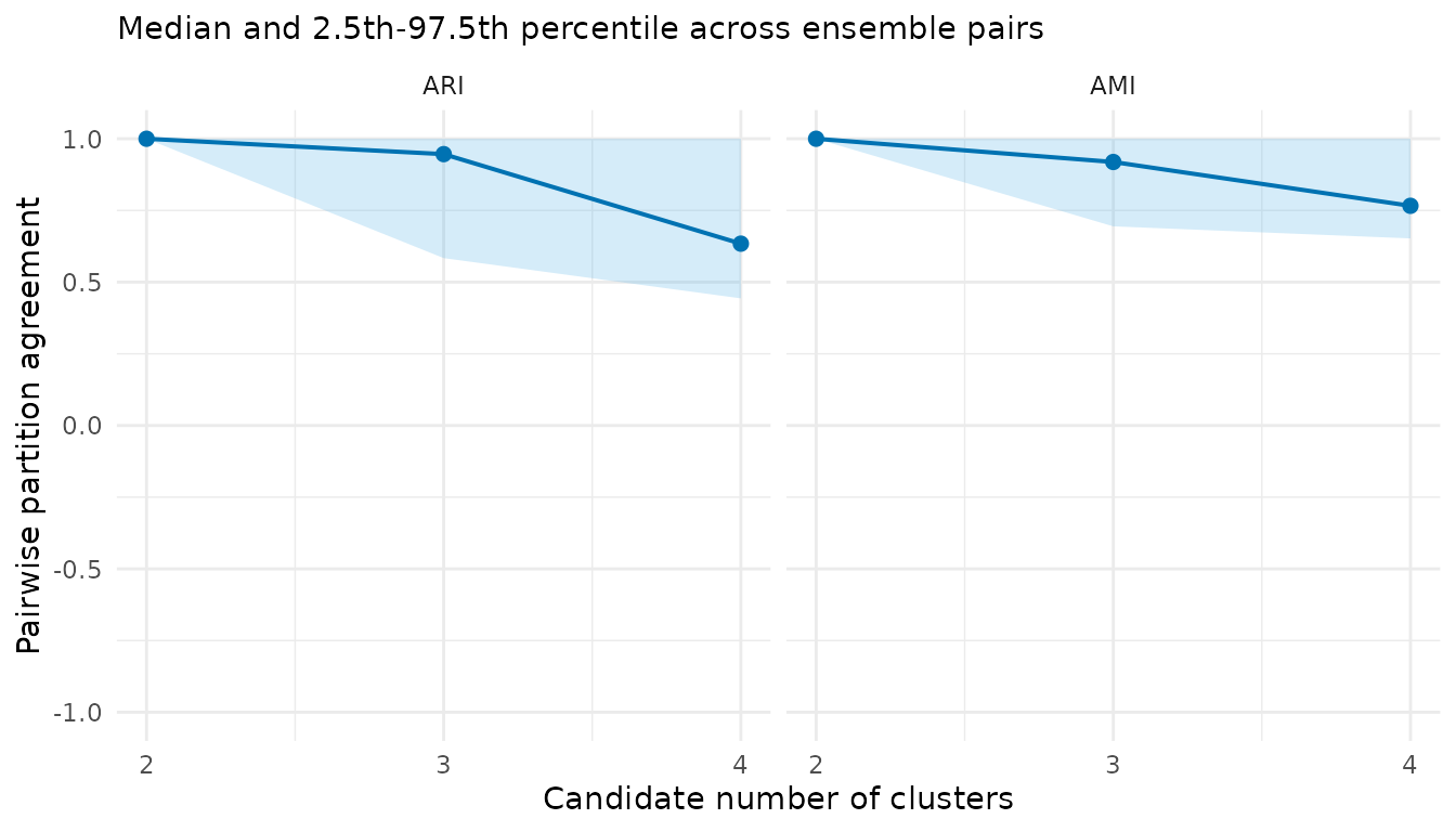
plot(transfer)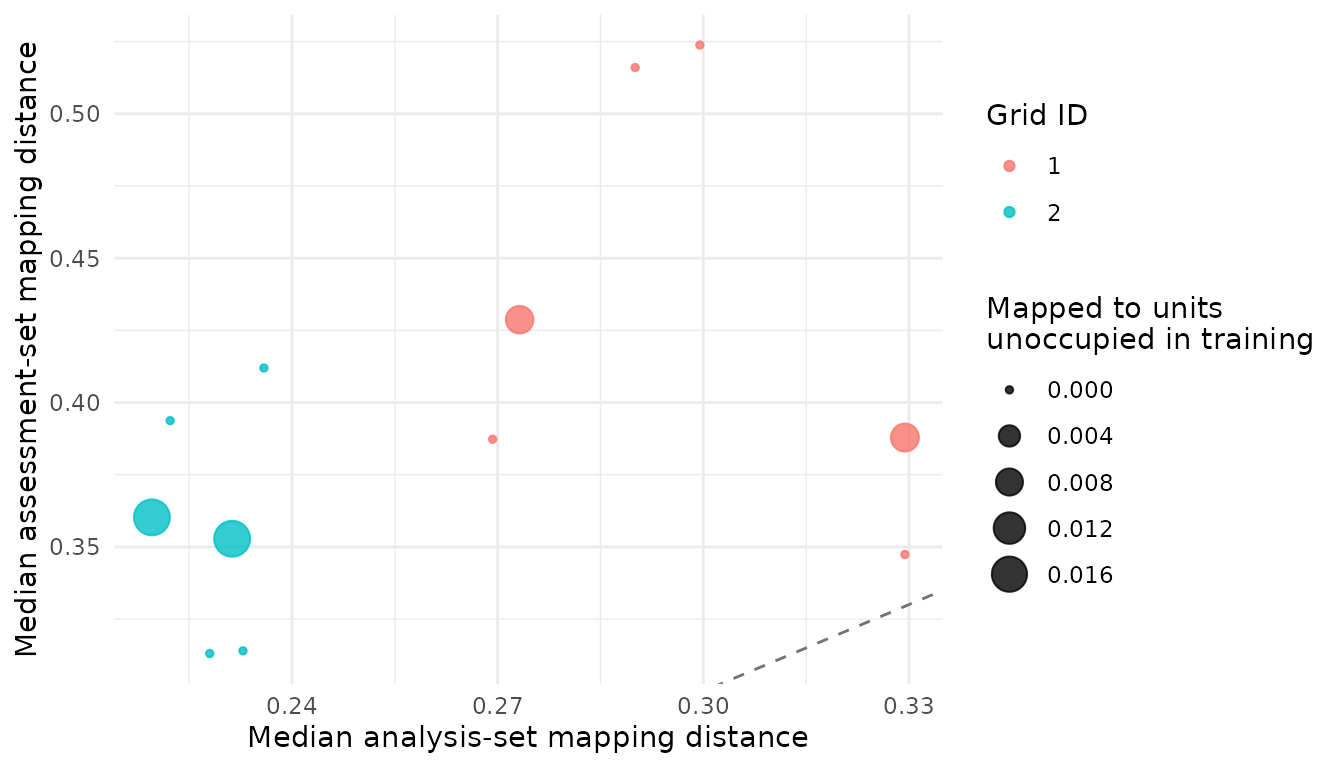
The map audit concerns representation. The partition plot concerns repeated hard classifications. The transfer plot concerns the held-out year. None is a classification-accuracy plot.
Compare with species after fitting
For this teaching example, inspect k = 3 because the
data contain three recorded species. This is a choice made before
viewing the agreement results. It is not evidence that
k = 3 is the best unsupervised partition.
consensus_k3 <- workflow$consensus$k3
external <- evaluate_external_labels(consensus_k3)

external
#> <som_external_assessment> (post hoc)
#>   samples used: 342 of 342
#>   label match : stored
#>   ARI         : 0.938
#>   AMI         : 0.912
#>   interpretation: agreement, not classification accuracy
external$contingency
#>                  external_label
#> consensus_cluster Adelie Chinstrap Gentoo
#>                 1    150         7      0
#>                 2      0         0    123
#>                 3      1        61      0
external$composition
#>   consensus_cluster external_label   n within_cluster_proportion
#> 1                 1         Adelie 150                0.95541401
#> 2                 2         Adelie   0                0.00000000
#> 3                 3         Adelie   1                0.01612903
#> 4                 1      Chinstrap   7                0.04458599
#> 5                 2      Chinstrap   0                0.00000000
#> 6                 3      Chinstrap  61                0.98387097
#> 7                 1         Gentoo   0                0.00000000
#> 8                 2         Gentoo 123                1.00000000
#> 9                 3         Gentoo   0                0.00000000
ARI, AMI and the contingency table describe agreement among the evaluable penguins. They do not prove that the partition is biologically correct. The main lesson is procedural: keep labels out of unsupervised training, then bring them back transparently for interpretation.
Save the record
Keep the exact data preparation, IDs, transfer design, SOM settings, warnings and failed fits with the result.
packageVersion("SOMevidence")
#> [1] '1.2.1'
packageVersion("palmerpenguins")
#> [1] '0.1.1'
sessionInfo()
#> R version 4.6.1 (2026-06-24)
#> Platform: x86_64-pc-linux-gnu
#> Running under: Ubuntu 24.04.4 LTS
#>
#> Matrix products: default
#> BLAS:   /usr/lib/x86_64-linux-gnu/openblas-pthread/libblas.so.3
#> LAPACK: /usr/lib/x86_64-linux-gnu/openblas-pthread/libopenblasp-r0.3.26.so;  LAPACK version 3.12.0
#>
#> locale:
#>  [1] LC_CTYPE=C.UTF-8       LC_NUMERIC=C           LC_TIME=C.UTF-8
#>  [4] LC_COLLATE=C.UTF-8     LC_MONETARY=C.UTF-8    LC_MESSAGES=C.UTF-8
#>  [7] LC_PAPER=C.UTF-8       LC_NAME=C              LC_ADDRESS=C
#> [10] LC_TELEPHONE=C         LC_MEASUREMENT=C.UTF-8 LC_IDENTIFICATION=C
#>
#> time zone: UTC
#> tzcode source: system (glibc)
#>
#> attached base packages:
#> [1] stats     graphics  grDevices utils     datasets  methods   base
#>
#> other attached packages:
#> [1] SOMevidence_1.2.1
#>
#> loaded via a namespace (and not attached):
#>  [1] gtable_0.3.6         jsonlite_2.0.0       kohonen_3.0.13
#>  [4] compiler_4.6.1       Rcpp_1.1.2           cluster_2.1.8.2
#>  [7] jquerylib_0.1.4      systemfonts_1.3.2    scales_1.4.0
#> [10] textshaping_1.0.5    yaml_2.3.12          fastmap_1.2.0
#> [13] ggplot2_4.0.3        R6_2.6.1             labeling_0.4.3
#> [16] knitr_1.51           palmerpenguins_0.1.1 tibble_3.3.1
#> [19] desc_1.4.3           bslib_0.12.0         pillar_1.11.1
#> [22] RColorBrewer_1.1-3   rlang_1.3.0          cachem_1.1.0
#> [25] xfun_0.60            fs_2.1.0             sass_0.4.10
#> [28] S7_0.2.2             otel_0.2.0           cli_3.6.6
#> [31] pkgdown_2.2.1        withr_3.0.3          magrittr_2.0.5
#> [34] digest_0.6.39        grid_4.6.1           lifecycle_1.0.5
#> [37] clue_0.3-68          vctrs_0.7.3          evaluate_1.0.5
#> [40] glue_1.8.1           farver_2.1.2         ragg_1.5.2
#> [43] rmarkdown_2.31       tools_4.6.1          pkgconfig_2.0.3
#> [46] htmltools_0.5.9